Time-domain solar wind noise
The solar wind imprints a time-variable dispersive delay on pulsar TOAs. PINT
can model the stochastic part of that delay in two different ways: as a
Fourier-basis Gaussian process, PLSWNoise,
or in the time-domain with a Gaussian process, TimeDomainSWNoise.
This page explains what the time-domain model infers, how it differs from the
Fourier-basis models that PINT uses and different choices for the interpolation basis and kernel.
For the general theory of correlated errors and the reduced-rank machinery that both families share, see Explanation under “Timing noise and correlated errors”.
What is actually being inferred
PINT’s deterministic solar wind component,
SolarWindDispersion, splits the
solar wind dispersion measure into an electron density and a purely geometric
factor:
Here \(n_E\) is the NE_SW parameter: the solar wind
electron number density in \(\mathrm{cm}^{-3}\), referenced to a distance
of 1 AU from the Sun. This is sometimes written as \(n_e(1\,\mathrm{AU})\). The density at any other radius is obtained from a
spherically symmetric power-law solar wind, which for the default SWM 0
(Edwards et al. 2006) is the usual \(1/r^2\) model,
so that the reference distance is just a normalization convention. The
geometry factor \(G(t)\) is the line-of-sight integral of that radial
profile through the wind at the epoch of each TOA; it is computed by
solar_wind_geometry()
and depends only on the pulsar’s solar elongation and the Earth-Sun distance,
not on any noise parameter. SWM 1 (Hazboun et al. 2022) generalizes the
radial index to a free parameter SWP, but the split is the same.
TimeDomainSWNoise makes the density a function of time. It places a
Gaussian process prior on
— the line-of-sight-averaged solar wind electron density, referenced to 1 AU under the same \(1/r^2\) model — and lets the existing geometry factor and the \(\nu^{-2}\) dispersion law carry it through to a delay:
where \(K\) is the dispersion constant pint.DMconst. The basis
matrix returned by
get_noise_basis() already
contains the \(G(t) K / \nu^2\) factor, so the Gaussian process
coefficients themselves are a density, in \(\mathrm{cm}^{-3}\).
Two practical consequences follow.
First, the amplitude hyperparameter TDSWLOGSIG is
\(\log_{10}\sigma\) with \(\sigma\) in \(\mathrm{cm}^{-3}\), not in
seconds. Physically sensible values are therefore of order
unity: TDSWLOGSIG 0.0 gives \(\sigma = 1\ \mathrm{cm}^{-3}\),
comparable to NE_SW itself.
Second, because the interpolation basis is a partition of unity (its rows sum
to one, see below), a constant set of GP coefficients is exactly equivalent
to a shift in NE_SW. The time-domain GP is best thought of as putting a
prior on the departures of the 1 AU density from its mean value or mean function.
Time domain vs. Fourier basis models
PINT’s existing stochastic components — PLRedNoise,
PLDMNoise, PLChromNoise,
PLSWNoise — are all Fourier basis models. They use
a Fourier design matrix \(F\) of sines and cosines at
frequencies \(k/T\), and a diagonal prior \(\phi\) whose entries are
the power spectral density evaluated at those frequencies. The process is
stationary by construction and its entire covariance structure is fixed by two
numbers, an amplitude and a spectral index.
TimeDomainSWNoise instead specifies the covariance directly as a function of
time lag. The basis \(U\) is a set of interpolation functions anchored at
nodes spread across the data span, and the prior can be a dense (2D)covariance
matrix \(K(t_i, t_j)\) evaluated at those nodes. In both cases the delay is
\(U a\) with \(a \sim \mathcal{N}(0, \Phi)\); what changes is what the
columns of \(U\) mean and whether \(\Phi\) is diagonal.
Spectral ( |
Time domain ( |
|
|---|---|---|
Basis columns |
sines and cosines at \(k/T\) |
interpolation functions at time nodes |
Prior \(\Phi\) |
diagonal; entries are the PSD |
dense covariance matrix \(K(t_i,t_j)\) |
Hyperparameters |
amplitude, spectral index ( |
amplitude, length scale, kernel shape |
Resolution set by |
number of Fourier modes ( |
node spacing ( |
Naturally expresses |
scale-free / power-law processes |
finite correlation times, periodicity, sharp features |
Stationary? |
always |
depends on the kernel |
The two descriptions are not rivals so much as different parameterizations of the same object: for a stationary process the Wiener-Khinchin theorem says the kernel \(K(\tau)\) and the PSD are a Fourier pair. What differs is which structures are easy to write down. A power law is trivial to state in the frequency domain and awkward in the time domain; a correlation that dies away after fifty days, or one that recurs on the solar cycle, is trivial in the time domain and requires many tuned Fourier modes to reproduce. The solar wind is a case where the time domain is the more natural language, since its variability is driven by solar activity with recognizable timescales rather than by a scale-free process. Moreover, the solar time series is better informed by TOAs at small solar elongations the time domain bases can more naturally parameterize around those epochs.
A few practical differences:
Edge behaviour. Fourier bases impose a lowest resolvable frequency \(1/T\) and are periodic over the span, which produces well-known leakage and edge artifacts. Interpolation bases have local support and no such periodicity.
Uneven sampling. Node spacing can be chosen (or set explicitly) to match the actual observing cadence, including gaps, rather than being tied to a uniform frequency grid.
Cost. The dense \(\Phi\) must be inverted, which
pint.utils.get_phiinv()does by Cholesky decomposition with a fallback to direct inversion. This is cheap as long as the number of nodes stays modest; the number of nodes, not the number of TOAs, sets the cost.
Because TimeDomainSWNoise is the first PINT component with a non-diagonal
\(\Phi\), the surrounding machinery — noise_model_basis_weight(),
the GLS fitters, pint.utils.woodbury_dot(),
pint.residuals.whiten_residuals() — accepts either a 1-D weight vector or
a 2-D covariance matrix. Models that mix diagonal and dense components get a
block-diagonal \(\Phi\), with one block per component.
The interpolation basis
The basis is built by pint.models.noise_model.make_interpolation_basis(),
which wraps scipy.interpolate.interp1d. Each column is the response of
one node: the function that equals one at that node and zero at every other
node, evaluated at the TOA epochs. For the default LINEAR interpolation
these are triangular “hat” functions.
import matplotlib.pyplot as plt
import numpy as np

from pint.models.noise_model import make_interpolation_basis

# One year of daily sampling.  PINT works in seconds internally, so that is
# what make_interpolation_basis expects; the nodes come back in seconds too.
t_mjd = np.arange(55000.0, 55360.5, 1.0)
t_sec = t_mjd * 86400.0

fig, (ax1, ax2) = plt.subplots(2, 1, figsize=(8, 6), sharex=True)

# --- (a) the linear interpolation basis itself ---
U, nodes = make_interpolation_basis(t_sec, dt=45.0, kind="linear")
for j in range(U.shape[1]):
    ax1.plot(t_mjd, U[:, j], lw=1.5)
ax1.plot(nodes / 86400.0, np.zeros_like(nodes), "k|", ms=16,
         label=f"{U.shape[1]} nodes, TDSWDT = 45 d")
ax1.plot(t_mjd, U.sum(axis=1), "k--", lw=1.2,
         label="row sum $\\equiv$ 1 (partition of unity)")
ax1.set_ylabel("basis value")
ax1.set_title("(a) Linear interpolation basis: one triangular 'hat' per node")
ax1.legend(loc="lower center", fontsize=8, ncol=2)
ax1.set_ylim(-0.08, 1.45)

# --- (b) the effect of TDSWINTERP_KIND on a single basis function ---
for kind in ("LINEAR", "NEAREST", "CUBIC"):
    # make_interpolation_basis passes `kind` straight to scipy, which wants
    # the lower-case spelling; the par file value is upper case.
    Uk, nodes_k = make_interpolation_basis(t_sec, dt=45.0, kind=kind.lower())
    j = Uk.shape[1] // 2
    ax2.plot(t_mjd, Uk[:, j], lw=1.8, label=f"TDSWINTERP_KIND = '{kind}'")
ax2.plot(nodes / 86400.0, np.zeros_like(nodes), "k|", ms=16)
ax2.axhline(0.0, color="0.75", lw=0.6, zorder=0)
ax2.set_xlabel("MJD")
ax2.set_ylabel("basis value")
ax2.set_title("(b) The same basis function under different interpolation kinds")
ax2.legend(fontsize=8, loc="upper right")
ax2.set_ylim(-0.35, 1.35)

fig.tight_layout()
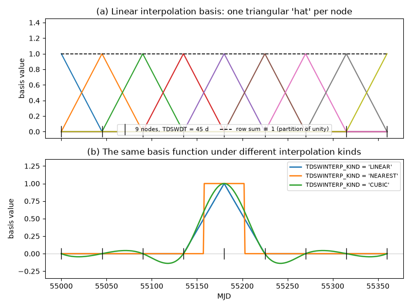
Three things about panel (a) matter for interpretation. The hats have local
support, so a node only influences TOAs within one spacing of it. They form a
partition of unity, so uniform coefficients reproduce a constant density —
this is why the GP is covariant with NE_SW. And columns with no support in
the TOA range are dropped, so the returned basis is automatically rank-reduced;
this is why a node placed outside the data span costs nothing.
Placing the nodes
There are two mutually exclusive ways to choose nodes, and validate()
rejects models that try to use both.
TDSWDTA uniform grid spacing in days, covering the TOA span. This is the default mode, with a default spacing of 30 days. Choosing it is a resolution trade-off: the spacing sets the shortest variation the model can represent, while the number of nodes sets the size of the dense covariance matrix that must be inverted. Solar wind work typically wants something in the range of one to a few weeks.
TDSWNODE_0001,TDSWNODE_0002, …Explicit node epochs in MJD, as prefix parameters. Use these when the cadence is uneven, when a specific set of epochs matters, or when nodes should be concentrated near solar conjunctions. At least two must be set, and their values must be finite and unique.
Nodes are most easily added with
add_tdsw_node_component(). Note that this callsvalidate()internally as soon as two nodes are present, so kernel parameters must be set before adding nodes.TDSWINTERP_KINDThe interpolation kind passed to
scipy.interpolate.interp1d; one ofLINEAR(default),NEAREST,NEAREST-UP,ZERO,SLINEAR,QUADRATIC,CUBIC,PREVIOUS, orNEXT. Panel (b) above shows the difference:NEARESTmakes the process piecewise constant, and the higher-order kinds trade smoothness for basis functions that overshoot and ring, undoing the strict locality and positivity of the linear hats.LINEARis the sensible default and the only one that is a partition of unity for arbitrary node spacing.
Kernels
TDSWKERNEL selects the covariance function evaluated at the nodes. Writing
\(\tau = |t_i - t_j|\), \(\sigma = 10^{\mathtt{TDSWLOGSIG}}\) in
\(\mathrm{cm}^{-3}\), \(\ell = 10^{\mathtt{TDSWLOGELL}}\) in days,
\(\Gamma_p = 10^{\mathtt{TDSWLOGGAMP}}\) and
\(P = 10^{\mathtt{TDSWLOGP}}\) in years, the four options are:
|
Required parameters |
\(K(\tau)\) |
|---|---|---|
|
|
\(\sigma^2 \delta_{ij}\) |
|
|
\(\sigma^2 \exp\left(-\tau^2 / 2\ell^2\right)\) |
|
|
\(\sigma^2 \exp(-\tau/\ell)\) for \(\nu=1/2\); \(\sigma^2 (1 + \sqrt{3}\tau/\ell)\exp(-\sqrt{3}\tau/\ell)\) for \(\nu=3/2\); \(\sigma^2 (1 + \sqrt{5}\tau/\ell + 5\tau^2/3\ell^2)\exp(-\sqrt{5}\tau/\ell)\) for \(\nu=5/2\) |
|
|
\(\sigma^2 \exp\left(-\tau^2/2\ell^2 - \Gamma_p \sin^2(\pi\tau/P)\right)\) |
All kernels except RIDGE add a small diagonal regulariser
\(d = (\sigma/50000)^2\) for numerical stability; the same trick, with a
different constant, is used in enterprise_extensions. The lag \(\tau\)
is computed in seconds internally, and the length scale and period are converted
from days and years respectively.
Choosing among them is a statement about how the density varies:
RIDGEIndependent fluctuations at each node — a white process, with no correlation between nodes at all. This is the default and the cheapest option, and it is the right choice when the node spacing is already the timescale of interest and you have no reason to impose smoothness. It gives a diagonal \(\Phi\), so it is effectively a per-epoch
NE_SWoffset with a Gaussian prior.SQEXPInfinitely differentiable, very smooth realizations with a single correlation timescale \(\ell\). Often too smooth for physical processes.
MATERNThe standard less-smooth alternative, with roughness controlled by \(\nu\) (
TDSWNU, one of 0.5, 1.5, or 2.5; default 1.5). Smaller \(\nu\) gives rougher realizations; \(\nu = 1/2\) is the Ornstein-Uhlenbeck process, and \(\nu \to \infty\) recoversSQEXP.QUASI_PERIODICA squared exponential multiplied by a periodic envelope: correlations recur with period \(P\) but decay over \(\ell\). This is the option that has no easy spectral analogue, and it is the natural way to express solar-cycle modulation (\(P \approx 11\) yr,
TDSWLOGP\(\approx 1.04\)) or annual structure. \(\Gamma_p\) sets how sharply the periodic part is enforced.
The plot below shows the correlation functions and one realization of the density from each.
import matplotlib.pyplot as plt
import numpy as np

from pint.models.noise_model import (
    make_interpolation_basis,
    matern_kernel,
    periodic_kernel,
    ridge_kernel,
    square_exponential_kernel,
)

rng = np.random.default_rng(42)

# Five years sampled daily, with interpolation nodes every 15 days.
t_mjd = np.arange(55000.0, 56825.5, 1.0)
t_sec = t_mjd * 86400.0
U, nodes = make_interpolation_basis(t_sec, dt=15.0, kind="linear")

LOGSIG = 0.3  # sigma = 2 cm^-3, comparable to NE_SW itself
kernels = [
    ("RIDGE", lambda n: ridge_kernel(n, LOGSIG)),
    ("SQEXP, $\\ell$ = 50 d", lambda n: square_exponential_kernel(n, LOGSIG, np.log10(50.0))),
    ("MATERN, $\\nu$ = 3/2, $\\ell$ = 50 d",
     lambda n: matern_kernel(n, LOGSIG, np.log10(50.0), 1.5)),
    ("QUASI_PERIODIC, $P$ = 1 yr",
     lambda n: periodic_kernel(n, LOGSIG, np.log10(300.0), 0.0, 0.0)),
]
colors = ["C0", "C1", "C2", "C3"]

fig, axes = plt.subplots(
    5, 1, figsize=(8, 9),
    gridspec_kw={"height_ratios": [2.0, 1, 1, 1, 1], "hspace": 0.32},
)

# --- (a) the kernels as correlation functions ---
ax = axes[0]
lag = np.linspace(0.0, 500.0, 601)
for (name, kfunc), color in zip(kernels, colors):
    row = kfunc(np.concatenate(([0.0], lag)) * 86400.0)[0]
    corr = row[1:] / row[0]
    if name == "RIDGE":
        # A pure delta function: zero at every non-zero lag.
        ax.plot([0, 0], [0, 1], color=color, lw=1.8)
        ax.plot(0, 1, "o", color=color, ms=5)
        ax.plot(lag, corr, color=color, lw=1.8, label=name + " (uncorrelated)")
    else:
        ax.plot(lag, corr, color=color, lw=1.8, label=name)
ax.set_xlabel(r"lag $\tau$ (days)")
ax.set_ylabel(r"$K(\tau)\,/\,K(0)$")
ax.set_title("(a) Kernel correlation functions")
ax.legend(fontsize=8)
ax.set_xlim(-8, 500)
ax.set_ylim(-0.05, 1.05)

# --- (b) one GP realization per kernel ---
for axi, (name, kfunc), color in zip(axes[1:], kernels, colors):
    K = kfunc(nodes)
    a = rng.multivariate_normal(np.zeros(len(nodes)), K)
    axi.plot(t_mjd, U @ a, color=color, lw=1.0)
    axi.axhline(0.0, color="0.75", lw=0.6, zorder=0)
    axi.set_ylabel(r"$\delta n_E$")
    axi.set_ylim(-8, 8)
    axi.text(0.012, 0.86, name, transform=axi.transAxes, fontsize=8,
             va="top", bbox=dict(fc="white", ec="0.8", alpha=0.85, pad=2))
    if axi is not axes[-1]:
        axi.set_xticklabels([])
axes[1].set_title(
    r"(b) GP realizations of $\delta n_E(t)$ in cm$^{-3}$"
    r" ($\sigma = 2$ cm$^{-3}$, nodes every 15 d)"
)
axes[-1].set_xlabel("MJD")

fig.subplots_adjust(top=0.95, bottom=0.06, left=0.11, right=0.98)
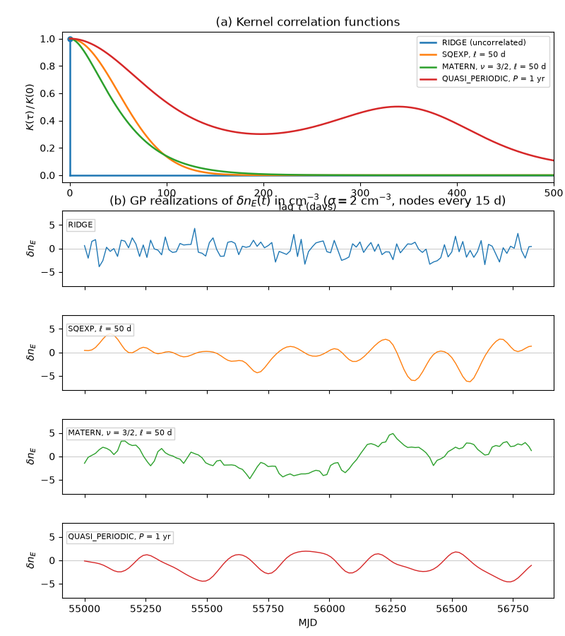
Note how different the four look at fixed \(\sigma\). The RIDGE
realization is jagged because neighboring nodes are independent and only the
interpolation ties them together; SQEXP is conspicuously smooth; MATERN
with \(\nu = 3/2\) wanders with visible short-timescale roughness; and the
quasi-periodic realization repeats on its period while slowly changing shape.
From density to observed delay
The geometry factor is what turns the inferred density into something the TOAs actually constrain, and it is strongly peaked in time. \(G(t)\) climbs steeply as the line of sight approaches the Sun, so it traces out a sharp cusp once a year at solar conjunction and is small and slowly varying the rest of the time. The delay is the product of that cusp with the smooth GP, which means the solar wind GP is informed almost entirely by TOAs taken near conjunction — and, through the \(\nu^{-2}\) law, by the lowest-frequency TOAs in the data set.
The figure below follows one realization through different views over five years, sampled densely enough to resolve the annual structure.
import astropy.units as u
import matplotlib.pyplot as plt
import numpy as np

from pint.config import examplefile
from pint.models import get_model
from pint.models.noise_model import TimeDomainSWNoise, square_exponential_kernel
from pint.simulation import make_fake_toas_uniform

LOGSIG = 0.0                  # sigma = 1 cm^-3
LOGELL = np.log10(200.0)      # 200 day correlation length

model = get_model(examplefile("B1855+09_NANOGrav_9yv1.gls.par"))

# Sample densely over five years at two widely separated frequencies, so that
# the annual solar conjunctions are resolved rather than aliased by the real
# observing cadence.
toas = make_fake_toas_uniform(
    53400, 53400 + 5 * 365.25, 1826, model,
    freq=np.array([430.0, 1400.0]) * u.MHz, obs="ao",
)

component = TimeDomainSWNoise()
model.add_component(component, validate=False)
model["TDSWKERNEL"].value = "SQEXP"
model["TDSWDT"].value = 15.0
model["TDSWLOGSIG"].value = LOGSIG
model["TDSWLOGELL"].value = LOGELL
model.validate()

mjd = toas.get_mjds().value
freq = model.barycentric_radio_freq(toas).to_value(u.MHz)
elong = model.sun_angle(toas).to_value(u.deg)

# DM_sw = n_E(t) * G(t), so the geometry factor carries all of the line-of-sight
# and 1/r^2 information.
geometry = model.solar_wind_geometry(toas).to_value(u.pc)

# One realization of the GP.  get_noise_basis folds in the geometry factor and
# the 1/nu^2 dispersion law, so B @ a is already a delay in seconds, while
# U @ a is the underlying density in cm^-3.
U, nodes = component._get_basis_and_nodes(toas)
B = component.get_noise_basis(toas)
rng = np.random.default_rng(4)
a = rng.multivariate_normal(np.zeros(len(nodes)), square_exponential_kernel(nodes, LOGSIG, LOGELL))
delay_us = (B @ a) * 1e6

lo = freq < 800  # the 430 MHz half of the simulated TOAs

fig = plt.figure(figsize=(11, 6.5))
gs = fig.add_gridspec(3, 2, width_ratios=[1, 2.1], hspace=0.18, wspace=0.25)
ax_geo = fig.add_subplot(gs[:2, 0])
ax_eq = fig.add_subplot(gs[2, 0])
ax_eq.axis("off")
ax_eq.text(
    0.5, 0.55,
    r"$\delta t \;=\; \delta n_E(t) \;\times\; G(t) \;\times\; K/\nu^2$"
    "\n\n(b)" r"$\;\times\;$" "(c)" r"$\;\rightarrow\;$" "(d)",
    transform=ax_eq.transAxes, ha="center", va="center", fontsize=10,
    bbox=dict(fc="0.96", ec="0.8", pad=6),
)
ax_ne = fig.add_subplot(gs[0, 1])
ax_g = fig.add_subplot(gs[1, 1], sharex=ax_ne)
ax_dt = fig.add_subplot(gs[2, 1], sharex=ax_ne)

# (a) why the geometry factor is cuspy: it climbs steeply toward conjunction
ax_geo.plot(elong, geometry, ".", ms=2, color="C4")
ax_geo.set_yscale("log")
ax_geo.set_xlabel("solar elongation (deg)")
ax_geo.set_ylabel(r"geometry $G$ (pc cm$^{3}$)")
ax_geo.set_title("(a) Line-of-sight geometry", fontsize=10)

# (b) the GP: a smooth, slowly varying density
ax_ne.plot(mjd[lo], (U @ a)[lo], color="C0", lw=1.4)
ax_ne.axhline(0.0, color="0.75", lw=0.6, zorder=0)
ax_ne.set_ylabel(r"$\delta n_E(t)$ (cm$^{-3}$)")
ax_ne.set_title(
    r"(b) The GP: a smooth density ($\sigma = 1$ cm$^{-3}$, $\ell$ = 200 d)",
    fontsize=10,
)
plt.setp(ax_ne.get_xticklabels(), visible=False)

# (c) the geometry factor in time: sharply peaked once a year
ax_g.plot(mjd[lo], geometry[lo], color="C4", lw=1.4)
ax_g.set_ylabel(r"$G$ (pc cm$^{3}$)")
ax_g.set_title("(c) ...times the geometry factor, which peaks at conjunction",
               fontsize=10)
plt.setp(ax_g.get_xticklabels(), visible=False)

# (d) their product: the observed delay
for band, color, label in [(lo, "C3", "430 MHz"), (~lo, "C2", "1400 MHz")]:
    ax_dt.plot(mjd[band], delay_us[band], color=color, lw=1.4, label=label)
ax_dt.axhline(0.0, color="0.75", lw=0.6, zorder=0)
ax_dt.set_xlabel("MJD")
ax_dt.set_ylabel(r"$\delta t$ ($\mu$s)")
ax_dt.set_title("(d) ...gives a delay with a sharp cusp every year", fontsize=10)
ax_dt.legend(fontsize=8, loc="upper left")

fig.subplots_adjust(left=0.07, right=0.99, top=0.94, bottom=0.09)
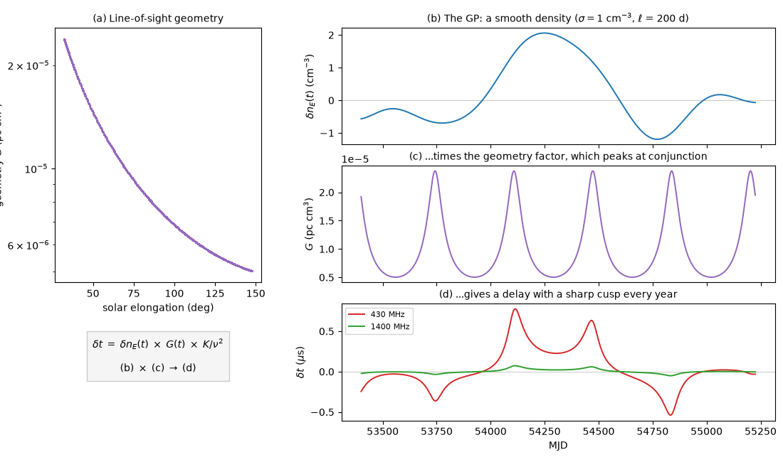
Panel (a) is for B1855+09, whose ecliptic latitude keeps it from ever coming closer than about 32 degrees to the Sun; a pulsar nearer the ecliptic reaches much larger geometry factors and is correspondingly better at constraining the wind. Panels (b) through (d) are the point of the figure. Notably, the Gaussian process itself is smooth and has no annual structure whatsoever — the periodicity in the delay is entirely geometric, imposed by \(G(t)\). What the GP controls is the amplitude and sign of each cusp: where \(\delta n_E(t)\) happens to be positive the conjunction produces a positive spike, and where it is negative the spike flips over. Two conjunctions a year apart can therefore look completely different, which is exactly the behavior a stationary power-law process in the Fourier basis struggles to reproduce.
Note also the frequency dependence: at \(\sigma = 1\ \mathrm{cm}^{-3}\) the 430 MHz cusps reach several hundred nanoseconds while the 1400 MHz curve stays almost flat, a contrast of roughly \((1400/430)^2 \approx 11\).
Using the component
TimeDomainSWNoise is selected automatically when a par file contains any of
its TDSW* parameters, and it round-trips through
get_model(). It can also be attached to an
existing model explicitly, which is convenient when building a model in Python.
Either way it requires a
SolarWindDispersion component in the
parent model, since that is where the geometry factor comes from.
from pint.models.noise_model import TimeDomainSWNoise

component = TimeDomainSWNoise()
model.add_component(component, validate=False)

model["TDSWKERNEL"].value = "MATERN"
model["TDSWDT"].value = 14.0
model["TDSWINTERP_KIND"].value = "LINEAR"
model["TDSWLOGSIG"].value = 0.0    # sigma = 1 cm^-3
model["TDSWLOGELL"].value = 1.5    # ell = 10^1.5 ~ 32 days
model["TDSWNU"].value = 1.5
model.validate()
which appears in the par file as:
TDSWKERNEL        MATERN
TDSWDT            14.0
TDSWLOGSIG        0.0
TDSWLOGELL        1.5
TDSWNU            1.5
TDSWINTERP_KIND   LINEAR
To use explicit nodes instead of a uniform grid, set every kernel parameter first and then add the nodes:
component = TimeDomainSWNoise()
model.add_component(component, validate=False)

model["TDSWKERNEL"].value = "RIDGE"
model["TDSWLOGSIG"].value = 0.0

for i, mjd in enumerate(node_mjds, start=1):
    component.add_tdsw_node_component(mjd, index=i)
model.validate()
Parameters
Name / Aliases |
Description |
Kind |
|---|---|---|
TDSWKERNEL |
Kernel for time-domain SW noise GP. Allowed values: ‘RIDGE’, ‘SQEXP’, ‘MATERN’, ‘QUASI_PERIODIC’. |
string |
TDSWDT |
Linear interpolation time step for time-domain SW noise. |
d |
TDSWLOGSIG |
Log10 amplitude of time-domain SW noise kernel. The GP coefficients are a solar wind electron density referenced to 1 AU, so sigma is in cm^-3 (not seconds). |
number |
TDSWLOGELL |
Log10 characteristic length scale for SQEXP / MATERN / QUASI_PERIODIC time-domain SW noise (days). |
number |
TDSWNU |
Matern smoothness parameter (supported: 0.5, 1.5, 2.5). |
number |
TDSWLOGGAMP |
Log10 mixing parameter for quasi-periodic time-domain SW noise. |
number |
TDSWLOGP |
Log10 periodicity of quasi-periodic time-domain SW noise (years). |
number |
TDSWINTERP_KIND |
Interpolation kind passed to scipy.interpolate.interp1d (upper case in the par file, lower-cased before the call). |
string |
TDSWNODE_{number} |
Interpolation node for time-domain SW noise basis (MJD). |
d |
References
Edwards, Hobbs & Manchester (2006), the
SWM 0\(1/r^2\) solar wind model: https://ui.adsabs.harvard.edu/abs/2006MNRAS.372.1549E/abstractHazboun et al. (2022), the
SWM 1variable-index solar wind model and stochastic solar wind modelling in PTA data: https://iopscience.iop.org/article/10.3847/1538-4357/ac5829Hazboun et al. (2026), time-domain Gaussian processes in PTA analyses: https://iopscience.iop.org/article/10.3847/1538-4357/ae4ee0
Rasmussen & Williams, Gaussian Processes for Machine Learning (2006), for the kernels themselves: https://gaussianprocess.org/gpml/